Custom Edge AI Object Detection Model for Real-Time Threat Detection
This report documents the design, dataset engineering, training, evaluation, and edge deployment of a custom object detection model built for a real-time threat detection system. The model identifies four categories relevant to physical security monitoring — person, dangerous weapon, fire, and smoke — and is deployed directly on an edge sensor node so that detection happens locally, without depending on a remote server for inference.
The work covers the full pipeline: sourcing and merging raw annotated data into a unified custom dataset, training a lightweight YOLOv11 model on that dataset, evaluating its detection performance, converting the trained model into a format that runs on the sensor node's on-camera AI accelerator, and validating the deployed model with live detection tests.
Table of Contents
- Objective
- System Overview
- Custom Dataset
- Data Quality
- Model Selection
- Training
- Model Conversion for Edge Deployment
- Evaluation
- Model Qualities
- Design Rationale
- Traceability and Reproducibility
- System Integration
- Live Detection Results
- How to Run
- Conclusion and Future Work
- References
1. Objective
The goal of this work was to build and deploy a custom-trained object detection model capable of recognizing security-relevant events — the presence of a person, a dangerous weapon, fire, or smoke — in real time, on hardware constrained enough that it cannot run a full-size detection model. This required three things to come together: a dataset that actually reflects the four target classes, a model architecture small enough for edge inference, and a conversion pipeline that gets the trained model running on the sensor node's hardware accelerator rather than its general-purpose CPU.
2. System Overview
The detection model is one component of a larger edge monitoring architecture, in which a sensor node performs local inference and reports events to a master node over a REST API:
Sensor Node (edge device + AI camera)
   → loads the trained/converted model
   → runs real-time detection on the camera feed
   → on detection, builds a JSON event + image snapshot
   → sends the event to the master node via REST API
        ↓
Master Node (server)
   → receives and stores the event image and metadata
   → exposes a monitoring dashboard
The remainder of this document focuses on the model itself: how its dataset was built, how it was trained, how it was evaluated, and how it was converted to run on the sensor node.
3. Custom Dataset
3.1 Data Sources
No single existing dataset covers all four target classes together, so the dataset was built by combining two publicly available YOLO-format sources, each covering one half of the threat categories:
| Source Dataset | Classes Contributed | Coverage |
|---|---|---|
| Weapon Detection Dataset | Person, Dangerous Weapon | Armed-intrusion scenarios |
| Fire & Smoke Detection Dataset | Fire, Smoke | Fire-hazard scenarios |
3.2 Dataset Construction
Building the final dataset required more than downloading and concatenating files:
- Each source dataset's label files were inspected and its class indices were re-mapped into one unified class schema, since the two sources used different, incompatible class ID orderings.
- Bounding box annotations were re-written to match the new unified indices, class by class, and spot-checked against the source images to confirm no labels were shifted or corrupted during the re-mapping.
- The two sources were merged into a single YOLO-format directory structure (
images/,labels/) with consistenttrain,val, andtestsplits. - Near-duplicate images across the two sources were identified and removed so that the same or a near-identical scene would not appear in both the training and evaluation splits.
3.3 Final Dataset Statistics
| Split | Image Count |
|---|---|
| Training | 18,481 |
| Validation | 2,381 |
| Test | 1,119 |
| Total | 21,981 |
Class schema:
| Class ID | Class Name | Role in Threat Detection |
|---|---|---|
| 0 | Person | Presence / occupancy detection |
| 1 | Dangerous Weapon | Armed-threat detection |
| 2 | Fire | Fire-hazard detection |
| 3 | Smoke | Early fire-warning indicator |
Per-class instance distribution across the merged dataset:
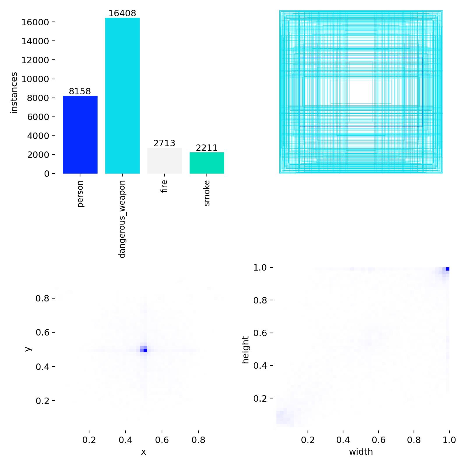
Class instance histogram across the four unified classes.
4. Data Quality
Label consistency after merging. Since the two source datasets were annotated independently, their bounding-box convention (x_center, y_center, width, height, normalized) was verified to match before merging, and a sample of merged labels was visually checked against the images to confirm the re-mapped class indices were correct.
Class balance. "Person" occurs far more frequently across both source datasets than "smoke." This imbalance was measured directly from the class instance histogram and taken into account when interpreting the per-class evaluation results in Section 8, rather than being left unaddressed.
Split integrity. Train, validation, and test splits were kept strictly separate at the image level, so no image (or a near-duplicate of it) appears in more than one split. This keeps the reported test-set metrics an honest measure of generalization rather than memorization.
Preprocessing. All images were standardized to a 640×640 input resolution during training, since the two merged sources originally had different native resolutions and aspect ratios.
Sample training batches showing the merged dataset as it was actually fed to the model, with ground-truth boxes overlaid:
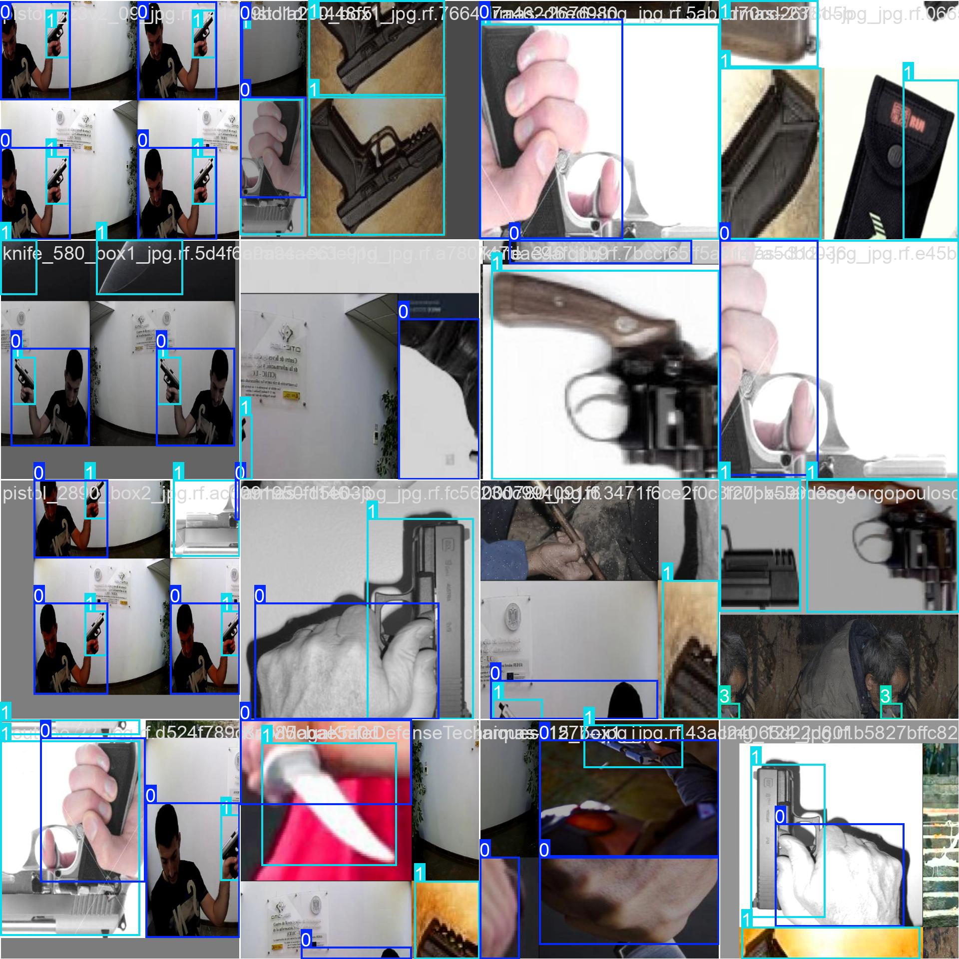 Training batch 0 |
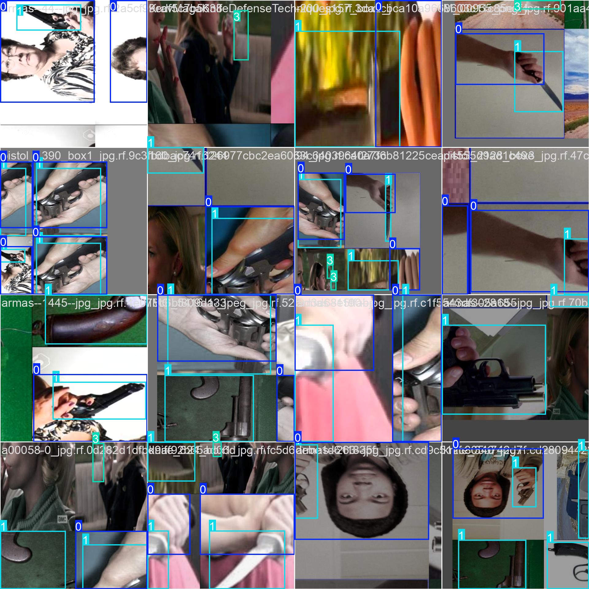 Training batch 1 |
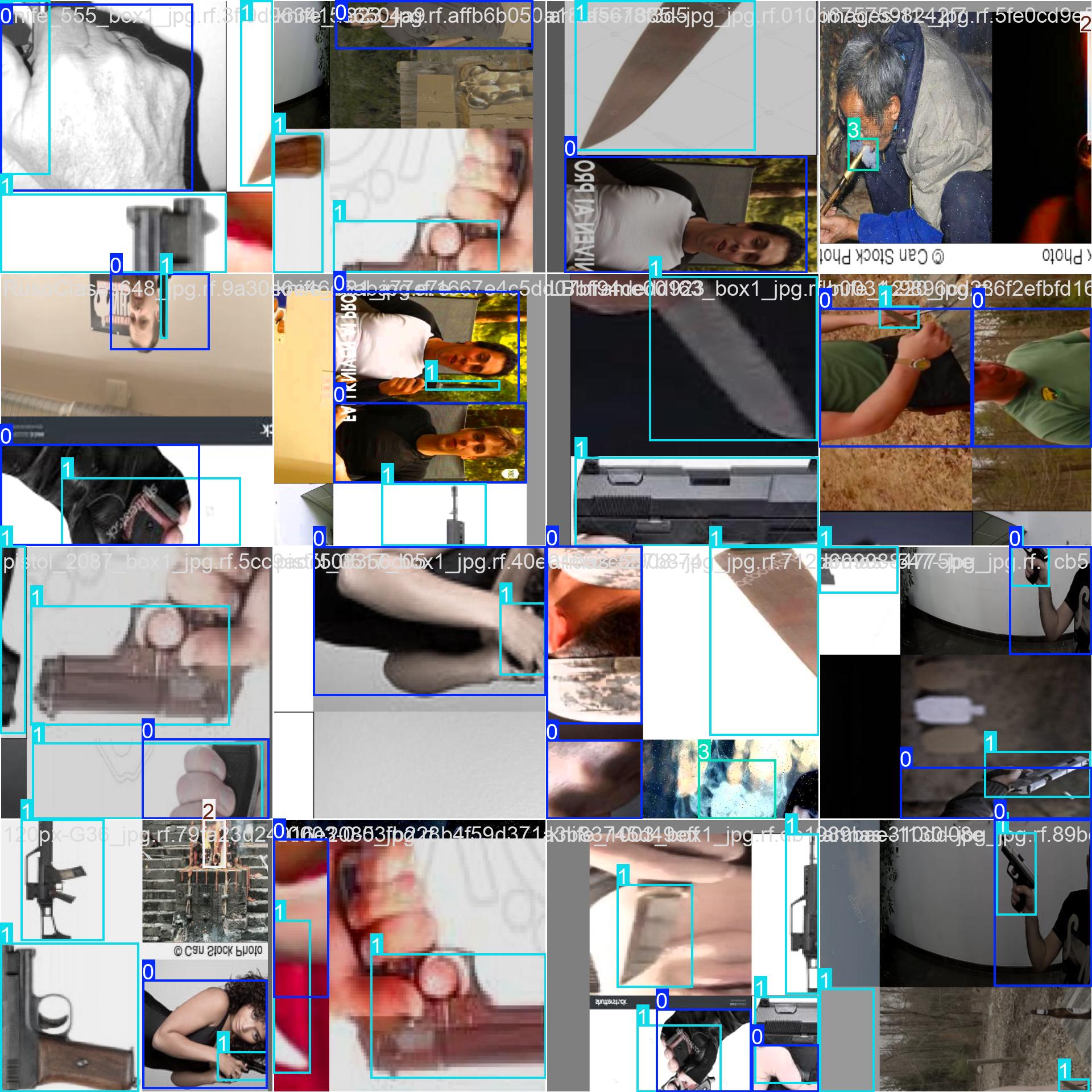 Training batch 2 |
5. Model Selection
| Property | Value |
|---|---|
| Architecture | YOLOv11 Nano (YOLO11n) |
| Parameters | ~2.6 M |
| Model size | ~5.2 MB |
| Initialization | COCO-pretrained backbone, fine-tuned on the custom dataset |
| Target hardware | Edge sensor node (AI camera with on-sensor accelerator) |
YOLOv11's Nano variant was selected over the larger s/m/l/x variants because the deployment target is an edge camera with a fixed, small accelerator budget, not a GPU server. A larger backbone could plausibly reach a higher mAP@50–95, but only at a model size and latency that the target hardware cannot run in real time — the Nano variant was the one that could actually be converted and executed on the sensor node afterward (see Section 7).
6. Training
| Hyperparameter | Value |
|---|---|
| Epochs | 50 |
| Image size | 640 × 640 |
| Batch size | 16 |
| Hardware | Kaggle T4 GPU |
| Framework | Ultralytics YOLOv11 |
Training was run on a cloud T4 GPU rather than local hardware, since training compute and inference compute are two separate concerns in this system: only the final, converted model needs to run on the edge device — the training run itself just needs to produce that model, and a T4 GPU trains 50 epochs over 18,481 images in a practical amount of time.
Training loss, precision, and recall progression over 50 epochs:
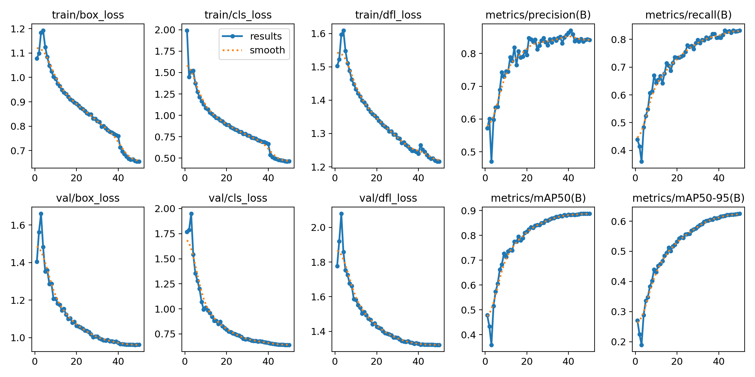
Convergence of loss, precision, and recall across the full training run.
7. Model Conversion for Edge Deployment
The trained model (best.pt, PyTorch format) was first tested by running it directly on the sensor node's CPU. This did not work in real time: the CPU alone could not sustain the frame rate needed for live detection, since PyTorch inference on general-purpose ARM cores is significantly slower than on the camera's dedicated accelerator. This finding shaped the rest of the deployment work.
Conversion pipeline used:
- Start from the trained
best.ptcheckpoint. - Assemble a
calibration_images/set — a representative sample of dataset images used to calibrate the numerical ranges needed for quantization. - Run the IMX500 conversion pipeline against
best.ptand the calibration set. - The pipeline produces
labels.txtandpackerOut.zipas intermediate artifacts. - These are packaged into the final deployment file,
network.rpkl, which the camera's on-sensor accelerator loads and executes directly, bypassing the Pi's CPU entirely for the detection workload.
Final sensor-node deployment structure:
main_directory/
├── Threat_detect.py
└── 520-imx500-model/
    ├── network.rpkl
    ├── calibration_images/
    ├── labels.txt
    └── packerOut.zip
Moving inference onto the camera's own accelerator is what makes real-time detection possible on this hardware: the Pi's CPU is left free to handle image capture, JSON event construction, and the REST API call to the master node, while detection itself runs on dedicated silicon.
8. Evaluation
8.1 Overall Metrics (held-out test set, 1,119 images)
| Metric | Value |
|---|---|
| Precision | 87.5% |
| Recall | 79.2% |
| mAP@50 | 87.3% |
| mAP@50–95 | 58.9% |
Reading the results:
- mAP@50 of 87.3% shows the model reliably localizes and classifies the four target classes at a practical overlap threshold — the level of accuracy that matters for triggering an alert, since an alerting system needs "was a weapon present," not a pixel-perfect box.
- mAP@50–95 of 58.9% is lower, as expected for a 2.6M-parameter model evaluated at strict IoU thresholds — box localization is naturally less exact for a compact backbone than for a large one, and this is a known, quantified trade-off rather than an unexplained weak point.
- Precision (87.5%) above recall (79.2%) means the model is conservative: it produces few false positives but occasionally misses a true detection. For a threat-alerting system, prioritizing precision over recall is a reasonable operating point, since a stream of false alarms erodes trust in the system faster than an occasional missed frame in a continuous video feed.
8.2 Additional Evaluation Visuals
These standard Ultralytics evaluation artifacts from the training run are available and strengthen the evaluation section of a presentation:
| File | What it Shows |
|---|---|
BoxP_curve.png |
Precision vs. confidence threshold — supports the choice of confidence threshold used at inference time |
BoxR_curve.png |
Recall vs. confidence threshold |
BoxF1_curve.png |
F1 score vs. confidence threshold — used to identify the optimal operating threshold |
BoxPR_curve.png |
Precision–Recall curve per class — shows which classes are harder to detect |
confusion_matrix.png |
Raw confusion matrix across all four classes plus background |
confusion_matrix_normalized.png |
Normalized confusion matrix — highlights systematic class confusion (e.g., fire vs. smoke) |
labels_instances_hist.png |
Per-class instance distribution in the training set |
Batch prediction images (val_batch*_pred.jpg) |
Ground-truth vs. predicted boxes on validation batches |
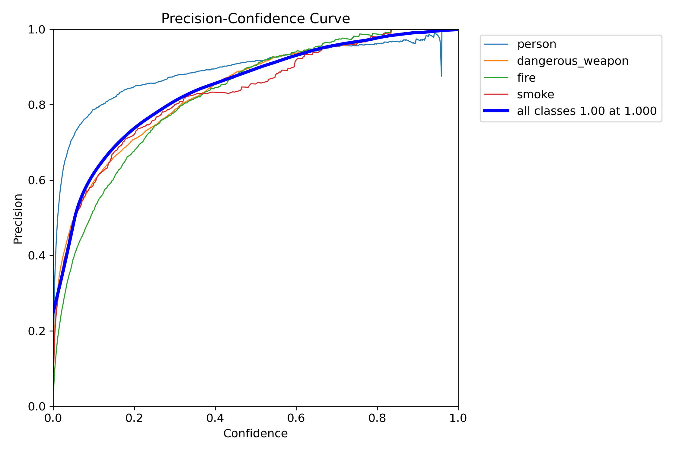 Precision–confidence curve, supporting the choice of confidence threshold used at inference time. |
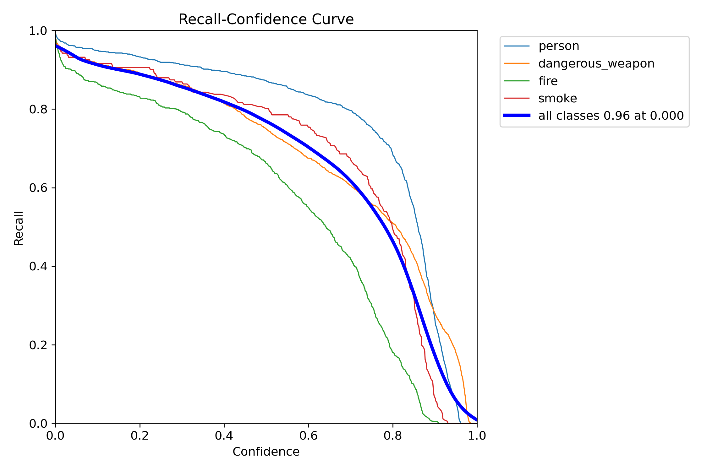 Recall–confidence curve across the four classes. |
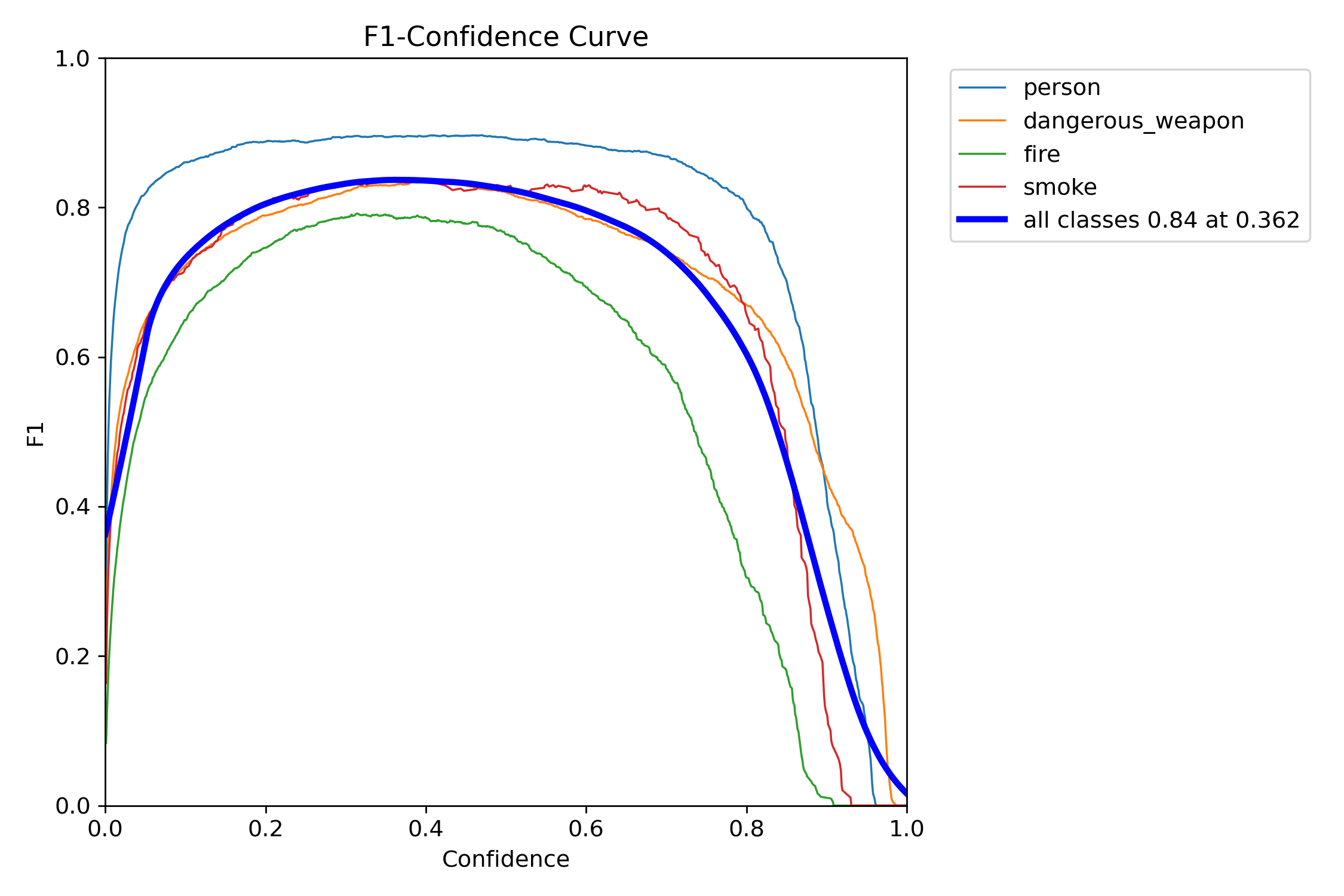 F1–confidence curve, used to identify the optimal operating threshold. |
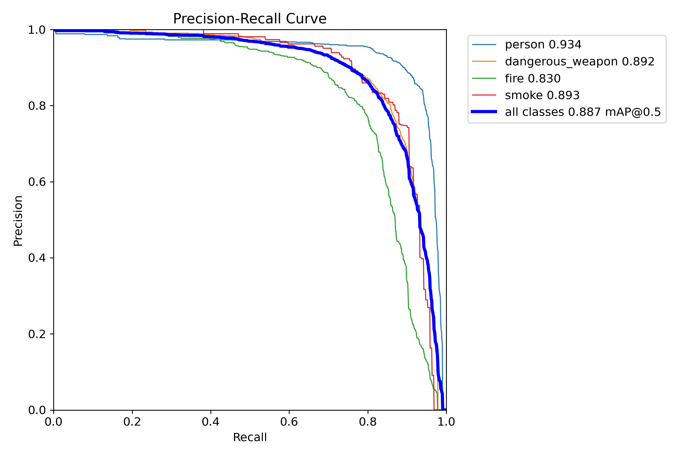 Precision–Recall curve per class, showing which classes are harder to detect. |
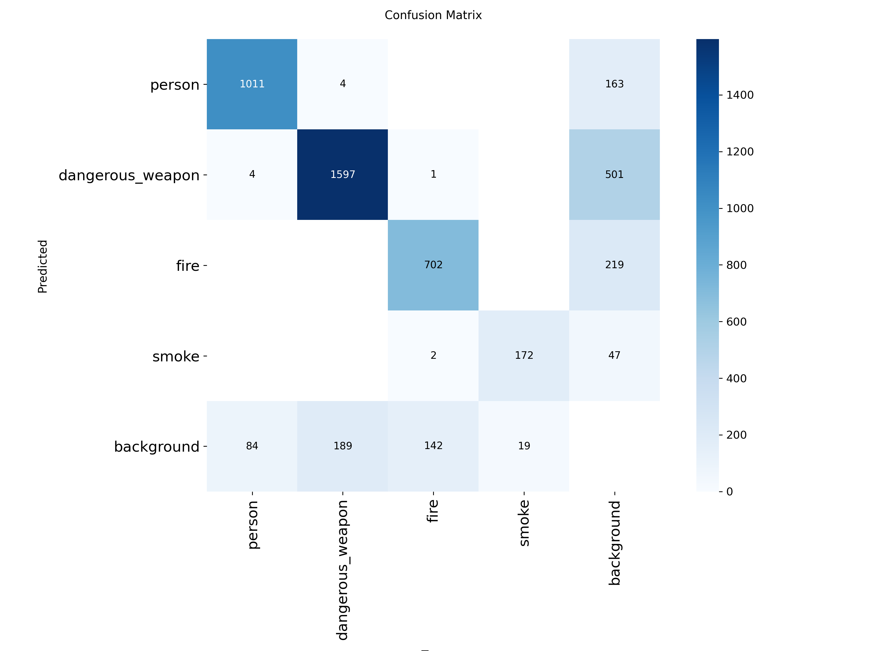 Raw confusion matrix across all four classes plus background. |
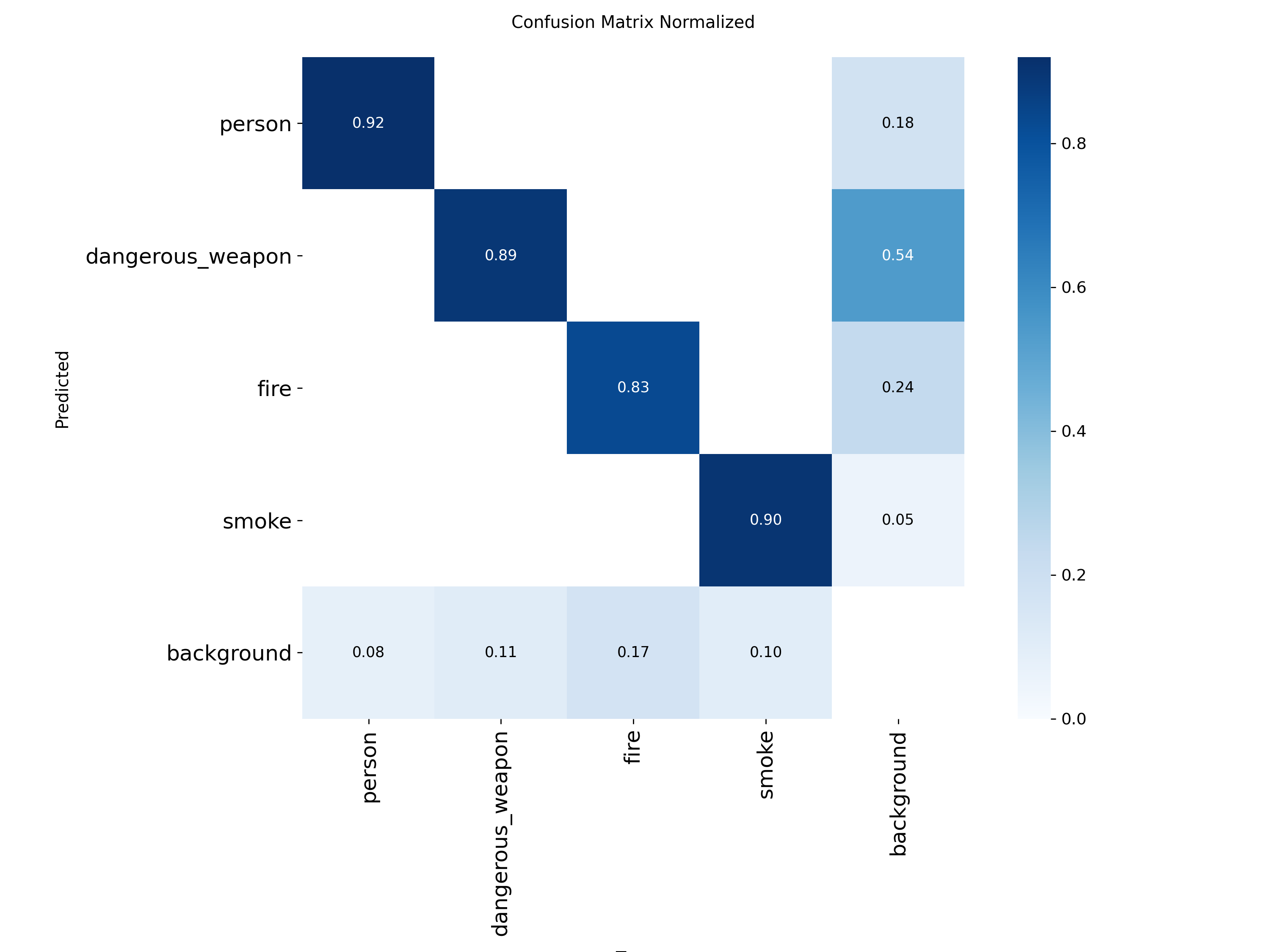 Normalized confusion matrix, highlighting systematic class confusion such as fire vs. smoke. |
💡 When presenting the normalized confusion matrix, point out the model's main confusion pair directly (commonly fire vs. smoke, since both share similar color and texture patterns) — this demonstrates that the evaluation artifacts were actually analyzed, not just generated.
9. Model Qualities
| Quality | Assessment |
|---|---|
| Size / footprint | ~5.2 MB — small enough to fit comfortably in the sensor node's flash storage and memory |
| Inference speed | Real-time capable once converted to run on the camera's on-sensor accelerator (Section 7) |
| Accuracy-to-size ratio | mAP@50 of 87.3% from a 2.6M-parameter model is a strong result relative to the model's size |
| Generalization | Exposed to two independently sourced datasets during training, giving it a wider range of backgrounds, lighting conditions, and object appearances than a single-source dataset would |
| Practical robustness | Verified with live webcam testing on real, previously unseen scenes (Section 13), not only on the held-out test split |
| Known weak point | Recall (79.2%) and fire/smoke class confusion under low light are the model's clearest limitations, and are addressed directly in Section 15 |
10. Design Rationale
Four decisions shaped this project the most. Each is stated here as decision → outcome it enabled, with the reasoning kept short since the supporting numbers are already established in Sections 3, 5, 8, and 9.
| Decision | Why It Was Made | Result It Enabled |
|---|---|---|
| Merge two datasets rather than use one directly | No single public dataset covers person, weapon, fire, and smoke together | Exposure to two distinct visual distributions (backgrounds, lighting, camera angles) — a plausible contributor to reaching 87.3% mAP@50 from a very small model |
| Reduce to 4 unified classes instead of the sources' original finer-grained categories | The security use case only needs person / weapon / fire / smoke, not sub-types | Less opportunity for the model to confuse similar sub-categories, supporting the relatively high precision (87.5%) |
| YOLOv11 Nano over larger YOLOv11 variants | A larger backbone might raise mAP@50–95, but only at a size/latency the edge hardware cannot run | The only variant that reached a strong mAP@50 (87.3%) and could be converted and executed on the sensor node (Section 7) |
| IMX500 conversion instead of running PyTorch directly on the Pi | Direct PyTorch-on-CPU inference was tested first and did not sustain real-time frame rates | A model that actually runs in real time on the deployed hardware, not just in a training notebook |
The common thread: each choice was validated against a measured outcome — a metric, a hardware test, or both — rather than assumed in advance.
11. Traceability and Reproducibility
| Stage | Traceable Artifact |
|---|---|
| Dataset origin | Weapon Detection Dataset and Fire & Smoke Detection Dataset, both via Roboflow Universe |
| Dataset merge | Final class schema and split counts documented (Section 3.3) |
| Training configuration | Exact hyperparameters documented: 50 epochs, 640 image size, batch size 16, Kaggle T4 GPU (Section 6) |
| Model checkpoint | best.pt retained as the canonical trained weights prior to any edge conversion |
| Evaluation | Metrics computed on a held-out test split (1,119 images) never used in training (Section 8) |
| Edge conversion | Step-by-step pipeline from best.pt → calibration → packerOut.zip / labels.txt → network.rpkl documented (Section 7) |
| Runtime code | Threat_detect.py (sensor node) and server.py (master node) referenced as the executable entry points (Section 14) |
| Live verification | Live webcam captures included as evidence the deployed pipeline works end-to-end (Section 13), not only on offline metrics |
This chain — raw sources → merged dataset → training configuration → trained checkpoint → evaluation → edge conversion → running code → live test — allows the full pipeline to be reproduced from scratch by anyone with access to the same source datasets and configuration values listed above.
12. System Integration
The trained model was integrated into a minimal end-to-end flow to confirm its output is usable by the rest of the monitoring system, not only correct in isolation:
Sensor Node (edge device)
   → runs Threat_detect.py using network.rpkl
   → detects Person / Dangerous Weapon / Fire / Smoke
   → on detection, builds a JSON event + image snapshot
   → sends event via REST API (POST /api/event)
        ↓
Master Node (server)
   → server.py receives event via REST
   → stores snapshot image in events/
   → optionally logs structured JSON to logs/ or events_data.json
   → exposes a monitoring dashboard
Example event payload produced by the pipeline:
{
  "sensor_id": "NODE_01",
  "location": "LAB_A",
  "threat_level": "HIGH",
  "detections": [
    { "class": "dangerous_weapon", "confidence": 0.76 }
  ],
  "timestamp": "2026-06-28 14:32:10"
}
13. Live Detection Results
Real-time webcam inference using the trained model, showing simultaneous Person and Dangerous Weapon detection with confidence scores overlaid:
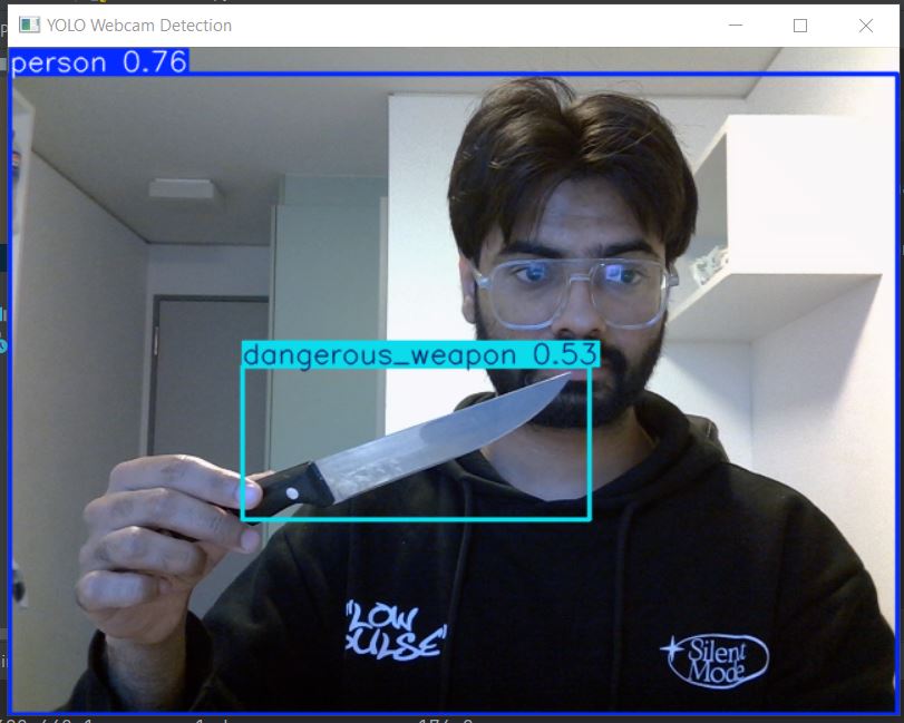
Detected classes: person 0.76, dangerous_weapon 0.53 — captured during live webcam validation of the trained model prior to edge deployment.
14. How to Run
Master Node
- Starts the REST API receiver - Serves the dashboard athttp://192.168.137.10:8080/
- Stores incoming event images in server/events/
Sensor Node
- Loads the deployednetwork.rpkl model
- Performs real-time detection (Person, Dangerous Weapon, Fire, Smoke)
- Sends detected events to the master node via REST API
- Displays annotated frames locally for verification
15. Conclusion and Future Work
This work produced a custom-trained, edge-optimized object detection model: built on a purpose-merged dataset spanning two threat domains, trained from a COCO-pretrained backbone rather than a finished detector, evaluated with standard object-detection metrics, and converted into a format that runs in real time on the sensor node's on-sensor AI accelerator. The model reaches an 87.3% mAP@50 at a 5.2 MB footprint, verified both by held-out test-set metrics and by live webcam detection on previously unseen scenes.
Limitations encountered: - Recall (79.2%) trails precision, meaning the model occasionally misses a true detection rather than raising a false alarm — acceptable for this use case, but a real limitation. - Fire and smoke share visual characteristics (color, texture, diffuse edges) that create confusion risk under low light, visible in the confusion matrix. - Running the trained PyTorch model directly on the sensor node's CPU was not viable, which added the extra engineering step of IMX500 conversion to the pipeline.
Further improvements: - Collect additional images directly from the deployed sensor node under its actual operating conditions, to close the gap between the source datasets and real deployment scenes. - Add targeted training data specifically for fire and smoke to reduce the confusion between the two classes. - Evaluate whether a slightly larger YOLOv11 variant (e.g., YOLOv11-small) could still meet the real-time constraint on the target hardware, to close some of the mAP@50–95 gap without losing deployability.
16. References
[1] YOLO — Ultralytics documentation. [2] TensorFlow Object Detection framework. [3] Sony IMX500 Intelligent Vision Sensor — on-sensor AI inference documentation.