Task 4 — Amdahl's Law & Gustafson's Law with Task Distributor

1. Introduction

Task 4 requires demonstrating Amdahl's Law and Gustafson's Law using a non-MPI parallel computing application. Task Distributor is a Bash-based parallel rendering tool that distributes a POV-Ray rendering job across multiple Raspberry Pi worker nodes (Cluster). In this project, the chess2.pov scene was used. The image is divided into horizontal strips, with each worker rendering one assigned strip. After all workers finish, the master node combines the strips into a single final image.

---

2. Infrastructure Overview

2.1 Cluster Hardware

Node	Hardware	Role
Master	Raspberry Pi 5	Coordinates benchmark execution, exports the shared NFS workspace, and composes the final rendered image.
Worker 1–8	Raspberry Pi 3 (905 MB RAM each)	Executes the assigned rendering task for its allocated image rows.

• The Raspberry Pi 5 acts as the central coordinator, responsible for task distribution, synchronization, result collection, and final image composition.
• Eight Raspberry Pi 3 devices execute the rendering tasks assigned by the master.
• SSH is used to remotely launch worker processes, while NFS provides a shared workspace for scene files, scripts, rendered image strips, and benchmark results.
• All experiments use the same POV-Ray scene (chess2.pov) to ensure consistent benchmarking conditions.

2.2 Dependencies Installed

The following software packages were installed to support distributed rendering, shared storage, timing measurements, and communication between the master and worker nodes.

Package	Installed on	Purpose
povray	Workers	Ray-tracing renderer — produces each row-strip of the scene
imagemagick (convert)	Workers + Master	Workers crop their row-strip; Master composes all strips into the final image
bc	Master	Floating-point arithmetic for timing (bash has no native float math)
nfs-kernel-server	Master	it could share a common workspace (/shared/povray) with all worker nodes
nfs-common	Workers	because workers mount and access that shared directory

Passwordless, key-based SSH from the master to all 8 workers is also required, since the master dispatches every worker's rendering job via SSH.

2.3 Shared NFS Workspace

The master exports one shared folder that every worker mounts identically:

/shared/povray/
├── scenes/chess2.pov              # the POV-Ray scene, read by every worker
├── task-distributor-worker.sh     # worker script, invoked over SSH
├── results_task_4.json            # accumulated timing results (all runs)
└── worker1.png … worker8.png      # each worker's rendered row-strip

Because this folder is shared, every worker sees the exact same files at the exact same path, and every worker writes its output back to the same place the master reads from.

---

3. Master Script

3.1 Row Distribution

The master divides the image into horizontal row ranges and assigns one range to each worker. For example, an image of 600 rows rendered by four workers is divided as:

Worker 1 → Rows   1–150
Worker 2 → Rows 151–300
Worker 3 → Rows 301–450
Worker 4 → Rows 451–600

3.2 Sequential Phase 1, Dispatch, and Completion Detection

Sequential Part 1 runs entirely on the master, before any worker starts rendering. In this phase, the master:

• Parses the command-line arguments (number of nodes, image width and height, shared path, law).
• Creates the lockfile on the shared NFS path.
• Calculates the row range each worker will be assigned

Dispatch: the master then gives each worker its instructions vsa SSH , passing the scene file and image width and height

Completion detection: each worker creates a small completion marker (workerX.done) after saving its image strip. The master periodically checks for these marker files and this is how the master knows all rendering is finished.

Sequential Phase 2 then master merges all the rendered image strips into a single final image using ImageMagick.

---

4. Worker Script

Each worker performs the following steps:

1. Receives its assigned row range from the master.
2. Renders only its assigned portion of the image using POV-Ray.
3. Saves the rendered image strip in the shared NFS directory.
4. Creates a completion marker (.done) so the master knows the worker has finished.

---

5. results_task_4.json — Data Collection

Every experiment run appends to this JSON file, structured as:

{
  "amdahl": {
    "results": [
      {
        "size": "800x600", "width": 800, "height": 600, "nodes": 4,
        "runs": 10, "average_runtime": 16.205,
        "speedup": 3.22, "efficiency": 80.5, "serial_fraction": 0.010966
      }
    ]
  },
  "gustafson": { "results": [ ... ] }
}

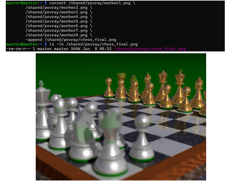
Final Rendered Image — Generated by 8 Workers

The image below is the final composed output produced when the scene was rendered using all 8 worker nodes — each worker rendered its assigned horizontal strip, and the master merged all 8 strips into this single final image.

---

6. Experiment 1 — Amdahl's Law 10 Runs × 6 Workloads

Amdahl's Law states that the overall performance improvement is limited by the serial portion of the program, even if we are adding more worker nodes.

Approach: for each of six fixed image sizes, vary node count across 1, 2, 4, and 8, holding the image size constant within each size group. This isolates the effect of adding processors to a fixed workload.

./task-distributor-master.sh -n 1 -x 800 -y 600 -p /shared/povray -l amdahl
./task-distributor-master.sh -n 2 -x 800 -y 600 -p /shared/povray -l amdahl
./task-distributor-master.sh -n 4 -x 800 -y 600 -p /shared/povray -l amdahl
./task-distributor-master.sh -n 8 -x 800 -y 600 -p /shared/povray -l amdahl

(repeated for 100×75, 200×150, 400×300, 1600×1200, 3200×2400 )

Amdahl's Law — Summary Table (Averages of 10 Runs)

Workload	Nodes	Avg Seq 1 (s)	Avg Parallel (s)	Avg Seq 2 (s)	Avg Total Time (s)	Speedup	Efficiency (%)
100x75	1	0.0043	3.112	0.0206	3.136	1.00	100.0
100x75	2	0.0029	2.806	0.0253	2.834	1.10	55.0
100x75	4	0.0027	2.108	0.0246	2.136	1.46	36.5
100x75	8	0.0022	2.220	0.0222	2.244	1.39	17.4
200x150	1	0.0066	5.117	0.0070	5.130	1.00	100.0
200x150	2	0.0536	4.007	0.0421	4.103	1.25	62.5
200x150	4	0.0028	3.009	0.0344	3.046	1.68	42.0
200x150	8	0.0019	3.532	0.0310	3.565	1.44	18.0
400x300	1	0.0027	14.221	0.0053	14.229	1.00	100.0
400x300	2	0.0023	9.015	0.0737	9.091	1.57	78.5
400x300	4	0.0025	5.912	0.0677	5.983	2.38	59.5
400x300	8	0.0023	4.015	0.0644	4.082	3.49	43.6
800x600	1	0.0029	52.171	0.0184	52.192	1.00	100.0
800x600	2	0.0022	29.742	0.1765	29.920	1.74	87.0
800x600	4	0.0027	16.027	0.1750	16.205	3.22	80.5
800x600	8	0.0023	9.925	0.1504	10.077	5.18	64.8
1600x1200	1	0.0030	211.093	0.0057	211.102	1.00	100.0
1600x1200	2	0.0029	113.356	0.7350	114.094	1.85	92.5
1600x1200	4	0.0031	59.387	0.8396	60.230	3.51	87.8
1600x1200	8	0.0027	32.454	0.7154	33.172	6.36	79.5
3200x2400	1	0.0029	793.297	0.0068	793.306	1.00	100.0
3200x2400	2	0.0022	434.201	3.4312	437.635	1.81	90.5
3200x2400	4	0.0021	222.408	2.6139	225.024	3.53	88.2
3200x2400	8	0.0029	117.475	1.8127	119.291	6.65	83.1

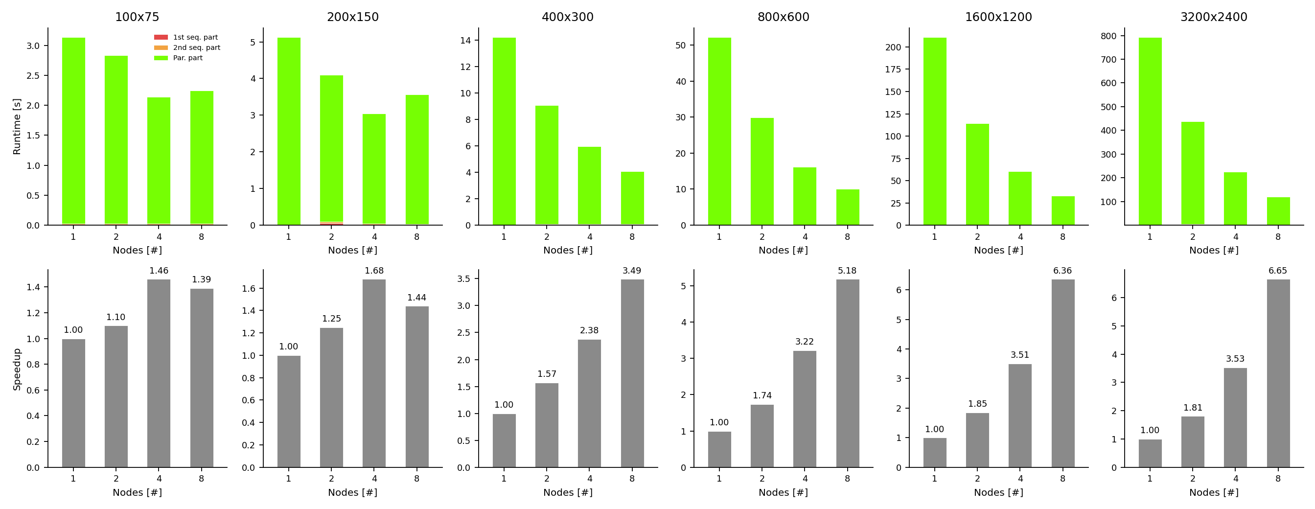
Graphs —Runtime & Speedup

Sequential Phase

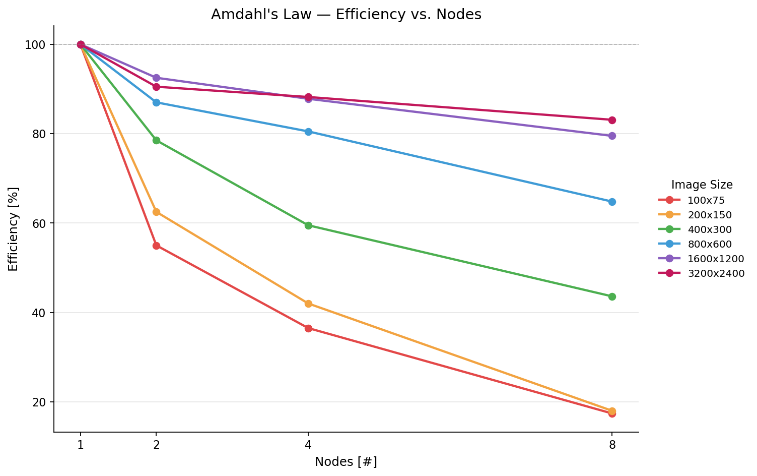
Efficiency vs. Nodes

Interpretation

With smaller image sizes, adding more nodes gives worse performance returns ( 100x75 and 200×150 ), probably because of SSH/NFS dispatch overhead becoming significant relative to the small rendering workload.

7. Experiment 2 — Gustafson's Law

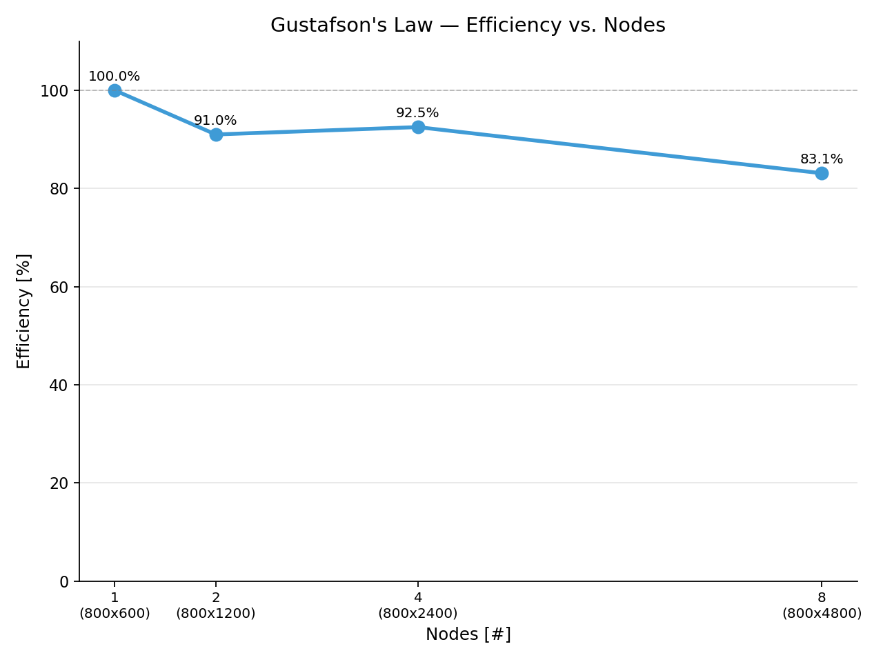
Gustafson's Law: Increase the problem size as we add more nodes. Each node performs approximately the same amount of work, so the sequential part becomes less important relative to the parallel workload, so allowing efficiently scaling

Approach: scale the image height in direct proportion to the node count (width fixed at 800), so each worker always renders approximately the same number of rows regardless of how many workers are used.

./task-distributor-master.sh -n 1 -x 800 -y 600  -p /shared/povray -l gustafson
./task-distributor-master.sh -n 2 -x 800 -y 1200 -p /shared/povray -l gustafson
./task-distributor-master.sh -n 4 -x 800 -y 2400 -p /shared/povray -l gustafson
./task-distributor-master.sh -n 8 -x 800 -y 4800 -p /shared/povray -l gustafson

(10 runs per configuration, 40 runs total)

Gustafson's Law — Summary Table (Average of 10 Runs per Configuration)

Workload	Nodes	Avg Seq 1 (s)	Avg Parallel (s)	Avg Seq 2 (s)	Avg Total Time (s)	Speedup	Efficiency (%)
800x600	1	0.0028	52.174	0.0056	52.182	1.00	100.0
800x1200	2	0.0021	56.980	0.3097	57.292	1.82	91.0
800x2400	4	0.0021	55.982	0.3974	56.382	3.70	92.5
800x4800	8	0.0020	62.095	0.6763	62.774	6.65	83.1

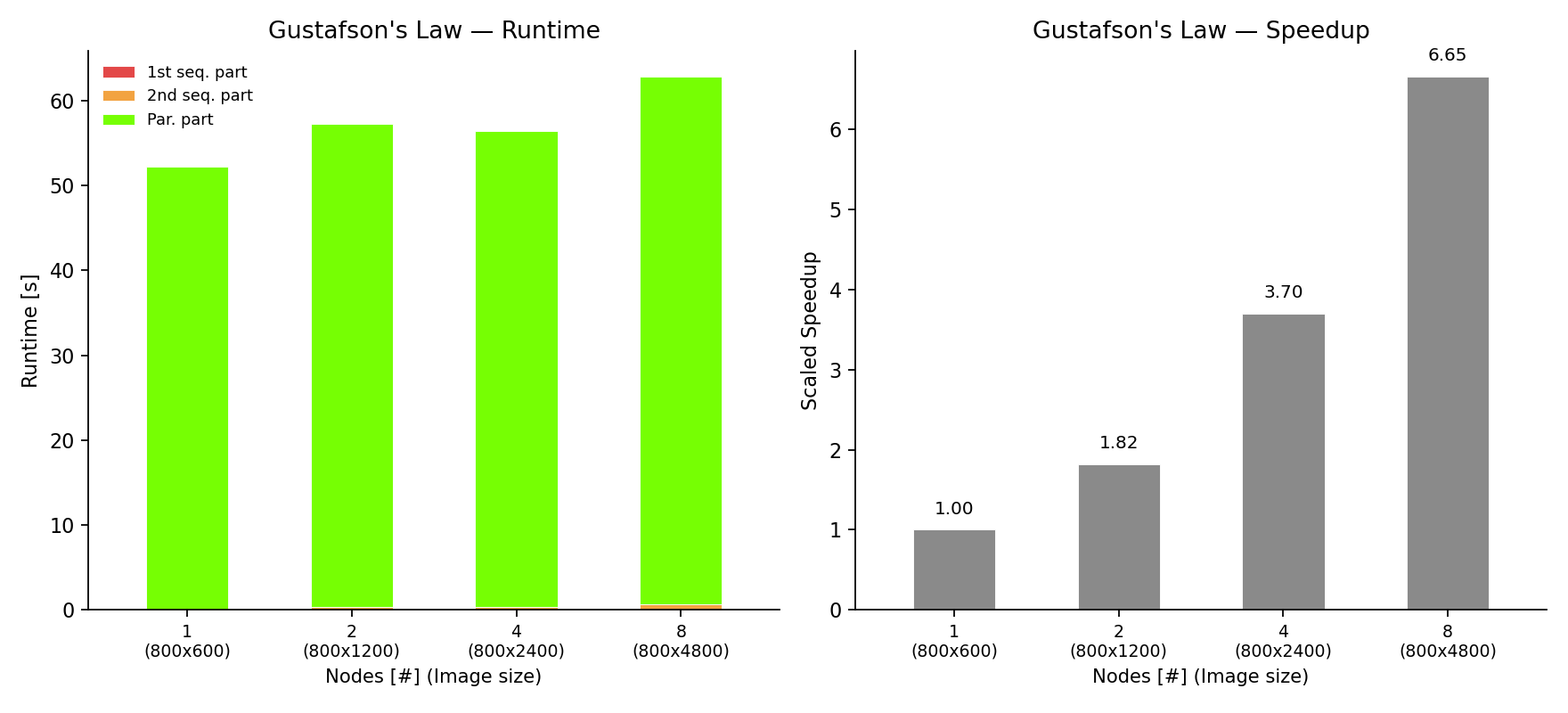
Graphs

Efficiency vs. Nodes

Interpretation

The results confirm Gustafson's Law: as the workload increases together with the number of nodes, each node processes approximately the same amount of work in a similar runtime, allowing the overall throughput and scaled speedup to increase nearly linearly

---

8. Limitation: RAM Constraints for Problem Size 6400×4800

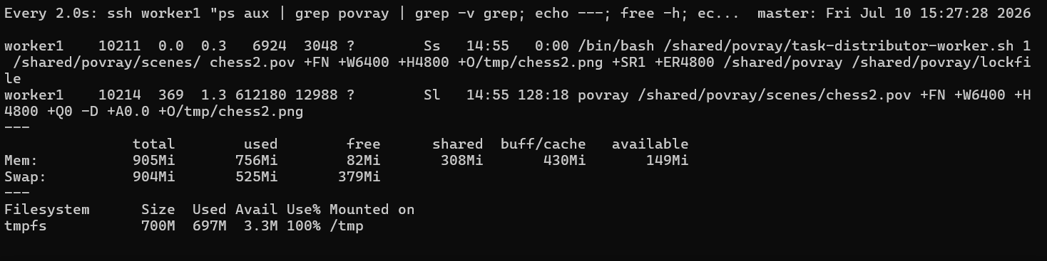
For the largest problem size (6400×4800), experiment was attempted during the Amdahl's Law. Since POV-Ray stores intermediate rendering image data in the RAM-backed /tmp (tmpfs) filesystem, the default /tmp allocation was increased from 453 MB to 700 MB to provide additional temporary storage. Despite this increase, reached 100% /tmp utilization (697 MB of 700 MB) after approximately 29 minutes of rendering, while the total rendering time was estimated to be approximately 53 minutes. At that point, the rendering process could not continue because the available temporary storage had been exhausted. Since /tmp is backed by the worker's limited physical memory, increasing its size further would only reduce the memory available for the operating system and other running processes. As result, the 6400×4800 workload could not be completed and was failed. This limitation indicate that the maximum problem size was constrained by the available RAM of the Raspberry Pi 3 worker nodes.

---

Cloud Computing Course SS2026 — Frankfurt University of Applied Sciences