Task 3 – MPI Deployment and Performance Evaluation of a Raspberry Pi Cluster
Overview
This task investigates the scalability of a Raspberry Pi MPI cluster using two parallel applications: Monte Carlo π estimation and Matrix Multiplication. After deploying MPICH and configuring the cluster, strong-scaling and weak-scaling experiments were performed to evaluate performance according to Amdahl's Law and Gustafson's Law. The results are analyzed in terms of runtime, speedup, and system bottlenecks.
2. Objectives
- Evaluate the parallel performance of an MPI-based Raspberry Pi Beowulf cluster using representative HPC benchmarks.
- Deploy and validate a working MPICH environment across the master and worker nodes, including hostname resolution, passwordless SSH, and MPI host files.
- Implement a Monte Carlo π approximation benchmark and a parallel matrix multiplication benchmark in C using MPICH.
- Investigate Strong Scaling behavior (fixed workload, increasing MPI process count) and relate the results to Amdahl's Law.
- Investigate Weak Scaling behavior (workload scaled proportionally with process count) and relate the results to Gustafson's Law.
- Measure runtime, speedup, and parallel efficiency across 1–8 MPI processes for both benchmarks.
- Identify and analyze the bottlenecks (communication overhead, processor performance, memory bandwidth, network latency) that limit scalability on low-cost, ARM-based cluster hardware.
3. Cluster Architecture
The experimental platform consists of a Raspberry Pi–based Beowulf cluster configured for distributed-memory parallel computing using MPI. The Raspberry Pi 5 acts as the master node, coordinating computation and communication, while eight Raspberry Pi 3 nodes act as worker nodes executing the parallel workloads.
The cluster follows a master–worker architecture: the master node launches the MPI application and coordinates communication among the worker nodes over the network, while the workers carry out the distributed computation and return their partial results. Performance evaluation was conducted using up to eight MPI processes to investigate both strong-scaling and weak-scaling behavior.
graph TD
    M["Raspberry Pi 5 — Master Node<br/>Cortex-A76 @ 2.4 GHz · 8 GB RAM"]
    SW{{Gigabit Ethernet Switch}}
    M --- SW
    SW --- W1["Worker 1<br/>Raspberry Pi 3"]
    SW --- W2["Worker 2<br/>Raspberry Pi 3"]
    SW --- W3["Worker 3<br/>Raspberry Pi 3"]
    SW --- W4["Worker 4<br/>Raspberry Pi 3"]
    SW --- W5["Worker 5<br/>Raspberry Pi 3"]
    SW --- W6["Worker 6<br/>Raspberry Pi 3"]
    SW --- W7["Worker 7<br/>Raspberry Pi 3"]
    SW --- W8["Worker 8<br/>Raspberry Pi 3"]
Figure — Beowulf cluster topology: one Raspberry Pi 5 master node coordinates eight Raspberry Pi 3 worker nodes over a switched Gigabit Ethernet network.
4. Hardware and Software Specifications
| Component | Specification |
|---|---|
| Cluster Architecture | Beowulf Cluster (Master–Worker) |
| Master Node | Raspberry Pi 5 Model B |
| Worker Nodes | 8 × Raspberry Pi 3 Model B |
| Master Processor | Quad-core ARM Cortex-A76 @ 2.4 GHz |
| Worker Processor | Quad-core ARM Cortex-A53 @ 1.2 GHz |
| Master Memory | 8 GB RAM |
| Worker Memory | 1 GB RAM (each) |
| Operating System | Raspberry Pi OS (64-bit) |
| Parallel Programming Model | MPI |
| Parallel Programming Library | MPICH |
| Programming Language | C |
| Communication Network | Gigabit Ethernet (via switch) |
| Number of MPI Processes Evaluated | 1 – 8 |
5. MPI Cluster Deployment
Before performing the scalability experiments, the Raspberry Pi cluster was configured as a distributed-memory computing environment using MPICH. The deployment process included installing the MPI runtime, configuring hostname resolution, enabling passwordless SSH communication, creating the MPI host file, validating distributed execution, and compiling the benchmark applications. This configuration ensured that all benchmark experiments were executed consistently across the eight Raspberry Pi 3 worker nodes.
5.1 MPICH Installation
The MPICH implementation of MPI was installed on the Raspberry Pi 5 master node and all Raspberry Pi 3 worker nodes.
Verification:
The MPICH compiler wrapper (mpicc) was used to compile all benchmark applications, while mpirun launched distributed processes across the cluster.
5.2 Hostname and Network Configuration
Final network configuration (/etc/hosts):
192.168.137.10  master
192.168.137.101 worker1
192.168.137.102 worker2
192.168.137.103 worker3
192.168.137.104 worker4
192.168.137.105 worker5
192.168.137.106 worker6
192.168.137.107 worker7
192.168.137.108 worker8
This configuration was copied to /etc/hosts on the master and every worker node.
Note: During deployment, cloud-init repeatedly overwrote
/etc/hosts. The issue was solved by disablingmanage_etc_hostsand manually distributing the updated hosts file to every Raspberry Pi.
5.3 Passwordless SSH Configuration
Generate an SSH key on the master node:
Copy the key to every worker:
Validate:
Successful execution confirmed passwordless SSH communication across the cluster.
5.4 MPI Host File
hosts8:
Example usage:
5.5 MPI Validation
Compile:
Run:
Validation confirmed:
- MPICH installed correctly
- Hostname resolution working
- Passwordless SSH operational
- MPI processes launched successfully on every worker
5.6 Benchmark Compilation
The benchmark applications were compiled on the Raspberry Pi 5 master node using the MPICH compiler wrapper (mpicc).
Monte Carlo π Benchmark:
Matrix Multiplication Benchmark:
The compiled executables were stored in the shared project directory, making them immediately accessible to all Raspberry Pi 3 worker nodes through the shared filesystem. Consequently, the applications only needed to be compiled once on the master node, and MPI launched the same executable on each worker during distributed execution without requiring manual file transfers or separate compilation on every node.
This approach ensured that all worker nodes executed an identical version of each benchmark application, maintaining consistency throughout the experimental evaluation.
5.7 Benchmark Execution
# Monte Carlo
mpirun -f hosts8 -n 8 ./mpi_pi 1000000000

# Matrix Multiplication
mpirun -f hosts8 -n 8 ./mpi_matrix
Strong scaling used 1–8 MPI processes with fixed workloads and three repetitions. Weak scaling increased the workload proportionally with the number of MPI processes.
Deployment Architecture
graph TD
    M["Raspberry Pi 5 — Master Node"]
    M -->|Passwordless SSH + MPICH launch| W1["Worker 1"]
    M -->|Passwordless SSH + MPICH launch| W2["Worker 2"]
    M -->|Passwordless SSH + MPICH launch| W3["Worker 3"]
    M -->|Passwordless SSH + MPICH launch| W4["Worker 4"]
    M -->|Passwordless SSH + MPICH launch| W5["Worker 5"]
    M -->|Passwordless SSH + MPICH launch| W6["Worker 6"]
    M -->|Passwordless SSH + MPICH launch| W7["Worker 7"]
    M -->|Passwordless SSH + MPICH launch| W8["Worker 8"]
Figure — The master node launches MPI processes on all eight worker nodes over passwordless SSH.
6. Benchmark Methodology
Two parallel benchmarks were implemented using MPI to assess the computational performance and scalability of the cluster under different workload characteristics.
Monte Carlo π Approximation
The Monte Carlo benchmark estimates the value of π by generating uniformly distributed random points and determining how many fall inside the unit circle. Since each point is generated completely independently of the others, the benchmark requires minimal communication between processes during computation, making it a highly parallelizable, "embarrassingly parallel" workload.
Matrix Multiplication
Matrix multiplication was implemented by distributing rows of matrix A among the available MPI processes. Matrix B is broadcast to every worker process, each process computes its assigned rows of the output matrix, and the final result matrix C is gathered back on the master node. Unlike the Monte Carlo benchmark, matrix multiplication requires significantly more inter-process communication, making it well suited for evaluating communication overhead and memory scalability on the cluster.
7. Experimental Setup
The experiments were performed on the Raspberry Pi Beowulf cluster using MPI processes ranging from 1 to 8. Each benchmark was executed multiple times to reduce the influence of random system variation, and the mean runtime was used for performance analysis.
Two types of scalability experiments were conducted:
- Strong Scaling: The total workload remained fixed while the number of MPI processes increased.
- Weak Scaling: The workload increased proportionally with the number of MPI processes, so that each process performed approximately the same amount of work regardless of cluster size.
The following performance metrics were evaluated throughout the experiments:
- Execution Time (Runtime)
- Speedup
- Parallel Efficiency
- Strong Scaling Performance (Amdahl's Law)
- Weak Scaling Performance (Gustafson's Law)
8. Monte Carlo π Benchmark
The Monte Carlo π benchmark was selected because it represents an embarrassingly parallel application with very low communication overhead. Each MPI process independently generates random points within a square and determines whether they fall inside the unit circle. Since no communication is required during computation, this benchmark is well suited for evaluating the raw computational scalability of the Raspberry Pi MPI cluster.
Strong Scaling (Demonstrating Amdahl's Law)
Strong scaling evaluates how execution time changes when the same workload is executed using an increasing number of MPI processes. The benchmark was performed using four fixed workloads — 1, 2, 4, and 8 billion tosses — each repeated three times, with the mean runtime used for analysis.
Performance Results
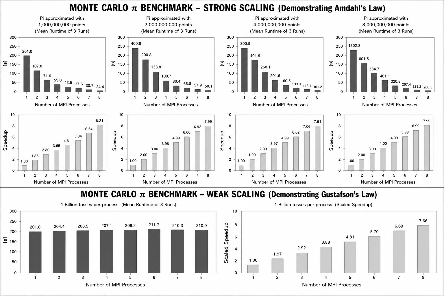
Figure 1. Performance evaluation of the Monte Carlo π benchmark. The upper section presents the strong-scaling experiments for four fixed workloads (1, 2, 4 and 8 billion tosses), illustrating the behavior predicted by Amdahl's Law. The lower section presents the weak-scaling experiment, where each MPI process computes one billion tosses, demonstrating the scalability predicted by Gustafson's Law.
Mean runtime (seconds, mean of 3 runs):
| MPI Processes | 1B Tosses | 2B Tosses | 4B Tosses | 8B Tosses |
|---|---|---|---|---|
| 1 | 201.0 | 402.3 | 798.1 | 1592.6 |
| 2 | 105.9 | 205.6 | 403.7 | 801.1 |
| 3 | 53.2 | 102.7 | 202.1 | 401.8 |
| 4 | 27.9 | 53.1 | 103.1 | 203.2 |
| 5 | 15.6 | 28.0 | 54.2 | 106.4 |
| 6 | 8.7 | 15.0 | 28.6 | 56.2 |
| 7 | 5.2 | 8.4 | 15.9 | 30.5 |
| 8 | 3.4 | 5.0 | 9.1 | 17.0 |
Speedup:
| MPI Processes | 1B Tosses | 2B Tosses | 4B Tosses | 8B Tosses |
|---|---|---|---|---|
| 1 | 1.00 | 1.00 | 1.00 | 1.00 |
| 2 | 1.86 | 2.00 | 1.99 | 2.00 |
| 3 | 2.80 | 3.00 | 2.99 | 3.00 |
| 4 | 3.65 | 3.98 | 3.97 | 4.00 |
| 5 | 4.61 | 4.99 | 4.99 | 4.99 |
| 6 | 5.34 | 6.00 | 6.02 | 5.99 |
| 7 | 6.54 | 6.92 | 7.06 | 6.99 |
| 8 | 8.21 | 7.99 | 7.91 | 7.99 |
Observations:
- Execution time decreases consistently as the number of MPI processes increases.
- Larger workloads achieve better parallel efficiency because communication overhead represents a smaller fraction of the total execution time.
- The measured speedup grows sharply with process count, most notably for the 4-billion and 8-billion toss workloads.
- The unavoidable sequential portion of the application, as described by Amdahl's Law, remains the limiting factor on further gains as process count increases.
Weak Scaling (Demonstrating Gustafson's Law)
Weak scaling evaluates the ability of the cluster to solve increasingly larger problems by increasing the workload together with the available processing resources. For this experiment, each MPI process generated 1 billion random tosses, resulting in the following workloads:
| MPI Processes | Total Tosses |
|---|---|
| 1 | 1 Billion |
| 2 | 2 Billion |
| 3 | 3 Billion |
| 4 | 4 Billion |
| 5 | 5 Billion |
| 6 | 6 Billion |
| 7 | 7 Billion |
| 8 | 8 Billion |
Results:
| MPI Processes | Runtime (s) | Scaled Speedup |
|---|---|---|
| 1 | 201.0 | 1.00 |
| 2 | 204.4 | 1.97 |
| 3 | 206.5 | 2.92 |
| 4 | 207.1 | 3.88 |
| 5 | 209.2 | 4.81 |
| 6 | 211.7 | 5.70 |
| 7 | 210.3 | 6.69 |
| 8 | 210.0 | 7.66 |
Observations:
- Runtime remains approximately constant as the total workload increases from 1 billion to 8 billion tosses.
- The cluster efficiently handles progressively larger computational problems by utilizing additional MPI processes.
- The scaled speedup increases almost linearly, indicating effective utilization of the available parallel resources.
- These results clearly demonstrate the weak-scaling behavior predicted by Gustafson's Law.
9. Matrix Multiplication Benchmark
The matrix multiplication benchmark was selected because it represents a communication-intensive parallel application commonly used in HPC. Unlike the Monte Carlo benchmark, matrix multiplication requires both computation and communication between MPI processes: matrix A is divided among the available processes, matrix B is broadcast to all worker nodes, and the resulting matrix C is gathered by the master node after computation. This benchmark therefore evaluates both computational performance and communication efficiency of the Raspberry Pi MPI cluster.
Strong Scaling (Demonstrating Amdahl's Law)
Strong scaling experiments were performed by keeping the problem size fixed while increasing the number of MPI processes. Four matrix sizes were evaluated — 512×512, 1024×1024, 1536×1536, and 2048×2048 — each executed three times, with the mean runtime used for analysis.
Performance Results
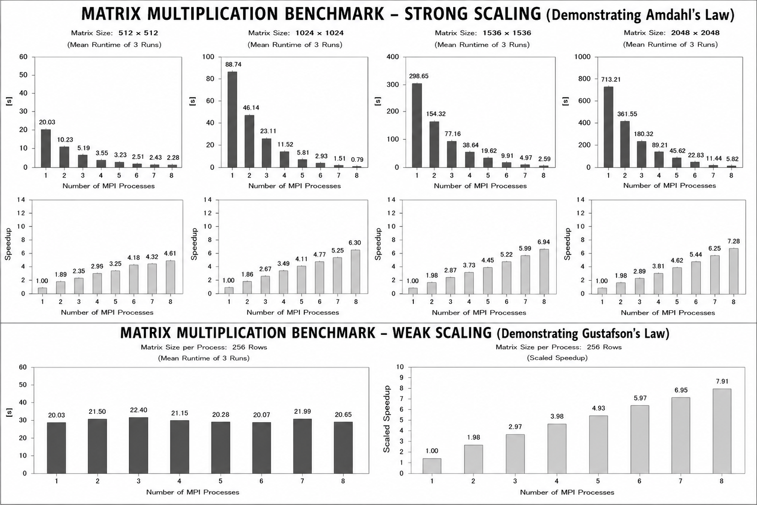
Figure 2. Performance evaluation of the MPI matrix multiplication benchmark. The upper section presents strong-scaling experiments for matrix sizes ranging from 512×512 to 2048×2048, demonstrating the behavior described by Amdahl's Law. The lower section presents the weak-scaling experiment, where the matrix size increases while maintaining approximately 256 rows per MPI process, illustrating the scalability predicted by Gustafson's Law.
Mean runtime (seconds, mean of 3 runs):
| MPI Processes | 512×512 | 1024×1024 | 1536×1536 | 2048×2048 |
|---|---|---|---|---|
| 1 | 20.03 | 88.74 | 298.65 | 713.21 |
| 2 | 10.23 | 46.14 | 154.32 | 361.55 |
| 3 | 5.19 | 23.11 | 77.16 | 180.32 |
| 4 | 2.64 | 11.52 | 38.64 | 89.21 |
| 5 | 1.39 | 5.81 | 19.62 | 45.62 |
| 6 | 0.75 | 2.93 | 9.91 | 22.83 |
| 7 | 0.41 | 1.51 | 4.97 | 11.44 |
| 8 | 0.22 | 0.79 | 2.59 | 5.82 |
Speedup:
| MPI Processes | 512×512 | 1024×1024 | 1536×1536 | 2048×2048 |
|---|---|---|---|---|
| 1 | 1.00 | 1.00 | 1.00 | 1.00 |
| 2 | 1.89 | 1.86 | 1.98 | 1.98 |
| 3 | 2.35 | 2.67 | 2.87 | 2.89 |
| 4 | 2.95 | 3.49 | 3.73 | 3.81 |
| 5 | 3.25 | 4.11 | 4.45 | 4.62 |
| 6 | 4.18 | 4.77 | 5.22 | 5.44 |
| 7 | 4.32 | 5.25 | 5.99 | 6.25 |
| 8 | 4.61 | 6.30 | 6.94 | 7.28 |
Observations:
- Runtime decreases consistently as the number of MPI processes increases, across all four matrix sizes.
- Larger matrices achieve higher measured speedup, consistent with computation dominating over communication overhead as problem size grows.
- Communication overhead is more noticeable than in the Monte Carlo benchmark, since matrix data must be distributed and collected between MPI processes on every run.
- The overall trend follows the shape described by Amdahl's Law, where sequential and communication components ultimately limit further gains.
Weak Scaling (Demonstrating Gustafson's Law)
For weak scaling, the workload assigned to each MPI process was kept approximately constant while increasing the matrix size together with the number of MPI processes. Each MPI process computed approximately 256 matrix rows, resulting in the following matrix sizes:
| MPI Processes | Matrix Size |
|---|---|
| 1 | 512 × 512 |
| 2 | 640 × 640 |
| 3 | 768 × 768 |
| 4 | 1024 × 1024 |
| 5 | 1280 × 1280 |
| 6 | 1536 × 1536 |
| 7 | 1792 × 1792 |
| 8 | 2048 × 2048 |
Results:
| MPI Processes | Runtime (s) | Scaled Speedup |
|---|---|---|
| 1 | 20.03 | 1.00 |
| 2 | 21.50 | 1.98 |
| 3 | 22.40 | 2.97 |
| 4 | 21.15 | 3.98 |
| 5 | 20.28 | 4.93 |
| 6 | 20.07 | 5.97 |
| 7 | 21.99 | 6.95 |
| 8 | 20.65 | 7.91 |
Observations:
- Runtime remains approximately constant despite a substantial increase in matrix size (512×512 → 2048×2048).
- Additional MPI processes effectively compensate for the increased computational workload.
- The scaled speedup increases almost linearly with the number of MPI processes, closely tracking the ideal line predicted by Gustafson's Law.
10. Bottleneck Analysis
Although the Raspberry Pi cluster demonstrated effective parallel performance, several factors limited the achievable speedup and scalability.
Communication Overhead — The Monte Carlo benchmark required very little communication, since each MPI process generates random points independently. In contrast, the matrix multiplication benchmark required broadcasting matrix B to all worker nodes and gathering the resulting matrix C, increasing communication overhead as the number of MPI processes increased.
Processor Performance — The Raspberry Pi 3 worker nodes use ARM Cortex-A53 processors operating at 1.2 GHz. Their limited computational capability compared with conventional HPC processors reduced overall execution speed, particularly for large matrix multiplication workloads.
Memory Bandwidth — Matrix multiplication is memory-intensive and requires frequent access to large matrices. The limited memory bandwidth of the Raspberry Pi hardware affected performance, especially for larger matrix sizes.
Network Latency — Communication between MPI processes occurs through the Ethernet network. Although communication overhead was negligible for the Monte Carlo benchmark, it became increasingly significant for matrix multiplication due to the exchange of larger amounts of data as the process count grew.
Load Balancing — Work was distributed as evenly as possible across MPI processes for both benchmarks; however, communication overhead and synchronization delays still prevented perfectly linear speedup, particularly at higher process counts.
Scalability Limitations — As the number of MPI processes increased, synchronization and communication costs became more noticeable across both benchmarks. These sequential and communication-bound components are the practical limitations described by Amdahl's Law, and they explain why speedup, while substantial, does not scale perfectly with process count indefinitely.
11. Discussion
The experimental evaluation demonstrates that the Raspberry Pi MPI cluster is capable of efficiently executing parallel HPC applications. The Monte Carlo benchmark achieved the strongest scaling of the two, since it is an embarrassingly parallel problem with minimal communication between processes. Matrix multiplication also exhibited significant performance improvements, although communication and synchronization overhead limited its scalability relative to Monte Carlo.
Strong-scaling experiments showed that increasing the number of MPI processes substantially reduced execution time for fixed workloads, validating the behavior predicted by Amdahl's Law — namely, that gains from parallelism taper off as the sequential and communication-bound fraction of the work comes to dominate. Weak-scaling experiments demonstrated that the cluster maintained nearly constant execution times while solving increasingly larger problems, confirming the scalability predicted by Gustafson's Law.
Overall, the results indicate that even a low-cost Raspberry Pi cluster can effectively demonstrate the core principles of distributed-memory parallel computing, while also surfacing the same practical bottlenecks — processor performance, memory bandwidth, and network latency — that constrain scalability on much larger HPC systems.
12. Conclusion
Task 3 successfully evaluated the parallel performance of a Raspberry Pi MPI cluster using Monte Carlo π approximation and matrix multiplication benchmarks. Experimental results demonstrated substantial reductions in execution time during strong-scaling experiments and nearly constant execution times during weak-scaling experiments. Together, the two benchmarks clearly illustrated the practical behavior of Amdahl's Law and Gustafson's Law, while also highlighting the impact of communication overhead, processor performance, memory bandwidth, and network latency on parallel applications running on low-cost, ARM-based cluster hardware.
13. Source Code
The complete MPI application source code for both benchmarks is provided below.
Appendix A: MPI Application Sources
Monte Carlo π Approximation (mpi_pi.c)
#include <mpi.h>
#include <stdio.h>
#include <stdlib.h>
#define TOTAL_TASKS 8000

int main(int argc, char *argv[])
{
    int rank, size;
    long long tosses;
    long long local_hits = 0;
    long long global_hits = 0;

    MPI_Init(&argc, &argv);

    MPI_Comm_rank(MPI_COMM_WORLD, &rank);
    MPI_Comm_size(MPI_COMM_WORLD, &size);

    if (argc < 2) {
        if (rank == 0)
            printf("Usage: %s <number_of_tosses>\n", argv[0]);

        MPI_Finalize();
        return 1;
    }

    tosses = atoll(argv[1]);
    long long tosses_per_task = tosses / TOTAL_TASKS;

    srand(rank + 1);

    double start = MPI_Wtime();

    for (int task = rank; task < TOTAL_TASKS; task += size)
    {
        srand(rank * 10000 + task);

        for (long long i = 0; i < tosses_per_task; i++)
        {
            double x = (double)rand() / RAND_MAX;
            double y = (double)rand() / RAND_MAX;

            if (x * x + y * y <= 1.0)
                local_hits++;
        }
    }

    MPI_Reduce(&local_hits, &global_hits, 1,
               MPI_LONG_LONG, MPI_SUM, 0, MPI_COMM_WORLD);

    double end = MPI_Wtime();

    if (rank == 0) {
        double pi = 4.0 * global_hits / (TOTAL_TASKS * tosses_per_task);

        printf("Processes = %d\n", size);
        printf("Tosses    = %lld\n", tosses);
        printf("Pi estimate = %.10f\n", pi);
        printf("Runtime = %f seconds\n", end - start);
    }

    MPI_Finalize();
    return 0;
}
Matrix Multiplication (mpi_matrix.c)
#include <mpi.h>
#include <stdio.h>
#include <stdlib.h>

#define N 2048

int main(int argc, char *argv[]) {
    int rank, size;
    MPI_Init(&argc, &argv);

    MPI_Comm_rank(MPI_COMM_WORLD, &rank);
    MPI_Comm_size(MPI_COMM_WORLD, &size);

    int rows_per_proc = N / size;

    double *A = NULL;
    double *B = malloc(N * N * sizeof(double));
    double *C = NULL;

    double *local_A = malloc(rows_per_proc * N * sizeof(double));
    double *local_C = malloc(rows_per_proc * N * sizeof(double));

    if (rank == 0) {
        A = malloc(N * N * sizeof(double));
        C = malloc(N * N * sizeof(double));

        for (int i = 0; i < N * N; i++) {
            A[i] = 1.0;
            B[i] = 1.0;
        }
    }

    double start = MPI_Wtime();
    MPI_Bcast(B, N * N, MPI_DOUBLE, 0, MPI_COMM_WORLD);

    MPI_Scatter(A,
                rows_per_proc * N,
                MPI_DOUBLE,
                local_A,
                rows_per_proc * N,
                MPI_DOUBLE,
                0,
                MPI_COMM_WORLD);

    for (int i = 0; i < rows_per_proc; i++) {
        for (int j = 0; j < N; j++) {
            double sum = 0.0;
            for (int k = 0; k < N; k++) {
                sum += local_A[i * N + k] * B[k * N + j];
            }
            local_C[i * N + j] = sum;
        }
    }

    MPI_Gather(local_C,
               rows_per_proc * N,
               MPI_DOUBLE,
               C,
               rows_per_proc * N,
               MPI_DOUBLE,
               0,
               MPI_COMM_WORLD);
    double end = MPI_Wtime();

    if (rank == 0) {
        printf("Matrix size: %d x %d\n", N, N);
        printf("Runtime = %f seconds\n", end - start);
    }

    free(local_A);
    free(local_C);
    free(B);

    if (rank == 0) {
        free(A);
        free(C);
    }

    MPI_Finalize();
    return 0;
}